How to Use the Site Storm Model

The M​odel My Watershed (MMW) Site Storm Model ​simulates storm runoff and water quality by applying the T​R-55 ​and S​TEP-L ​water quality models for a single 24-hour rain storm over a selected land area within the continental United States. The results are calculated based on actual land cover data (from the U​SGS National Land Cover Database 2011, ​NLCD2011) and actual soil data (from the U​SDA Gridded Soil Survey Geographic Database, ​gSSURGO) for the selected land area of interest. The complementary MMW M​icro ​Site Storm Model performs the same model calculations on a hypothetical land parcel with a single land cover class and a single hydrologic soil group.

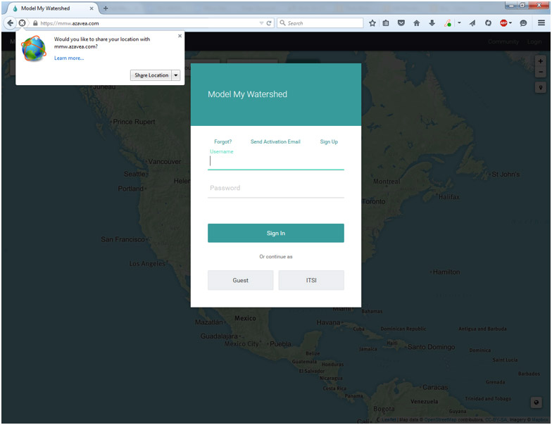
The MMW Site Storm Model can be accessed online from any web browser at mmw.azavea.com ​or through the through the I​nnovative Technology in Science Inquiry (ITSI) portal. ​When you first navigate to the MMW application, depending on your browser's settings you may be asked to share your location data with the application. Sharing your location will automatically start the application at approximately your current location, but is not necessary for the application to work. You will also immediately be given a chance to sign in to the application. Signing in allows you to save your work to return to later and to share your work with other users. For users who have registered on the site before, simply type in your username and password and click "Sign In." New users can create a sign in by clicking "Sign Up" in the upper right. For students and teachers who are using the Innovative Technology in Science Inquiry (ITSI) portal, click the "ITSI" button. This will verify your credentials for the ITSI portal and prevent you from needing to set up a new user for the application. This also allows you to quickly and easily send data and screenshots back and forth to assignments and lessons on the ITSI portal. For anyone who does not need or want to save data, you can simply click the “Guest” button and continue without any credentials. Logging in as a guest gives you access to the full modeling and scenario capabilities of the application, but will you not be able to save and share any data or easily send it to the ITSI portal.

Once you have logged into the application, you will see a map looking much like Google maps. If you shared your location, the application may zoom directly to your location, otherwise it will begin by showing a map of the entire U.S. As with most online map tools, you can navigate the map by clicking and dragging and zoom by pinching, using a scroll wheel, or using the zoom buttons on the upper left. You can also search for a location by name or address using the "Search" box on the upper left. To go or return to your current location, hit the “My Location” button with a picture of a pin below the zoom buttons on the upper left.

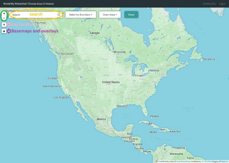
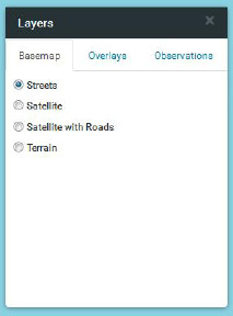
Just as Google maps allows you to switch between road and satellite maps, there are several options for both the base map and data overlays on top of the map. To access these click the button that looks like a small globe on the upper left. You can select a the basemap image and several different types of overlays. The base maps themselves come directly from ESRI or Google Maps and are not built into the application. If you have a very slow Internet connection, the base maps may be slow to load. The overlays include boundary lines (like school districts and USGS hydrologic units) and color shading for land uses and soil types. There are also observation data overlays, which display locations and data from the USGS and other national river and weather monitoring stations. Please note that observation data is not available in all locations!

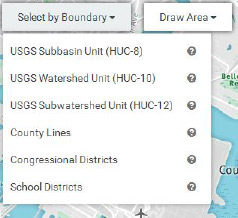
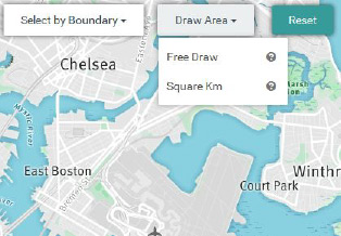
To begin modeling, you must first select a map area to model over. Do this with either the “Select by Boundary” or the “Draw Area” tool on the top part of the map (next to the search bar). You can select by political (county lines, congressional districts, and school districts) or major watershed (HUC 8-12) boundaries in the “Select by Boundary” tool. Once you have selected a boundary type those borders will appear on the map and the name of each region will appear as you hover over it. Be aware of your zoom level when selecting by boundaries. If you are at too high of a zoom level, you may not be able to see the boundaries on your map. You can use the “Draw Area” tool to draw a precise area of any size you want by drawing points on the map and double clicking or clicking on the first point to close the box. You can also use the “Draw Area” tool to select a 1 km box centered where ever you click.

As soon as you have selected an area or closed the box of your custom area the application will change into geospatial analysis mode. The left side of the screen will now show the area you selected in bright colors with the rest of the map greyed out. The right side of the screen will show two panes, one with analysis of the existing land cover and soil types in your selected area, the other with the option of running a model to predict runoff and nutrient loads for the area. These calculations and analysis are done on the fly for each area based on nationally available data. You will n​ot ​get some pre-computed estimate or “canned” number. These are real values based on the most recently available national land cover and soil type datasets. Because of this, the analysis may take a few seconds to compete and you may see a loading wheel on the right portion as this happens. (It is generally very fast with a good Internet connection.)

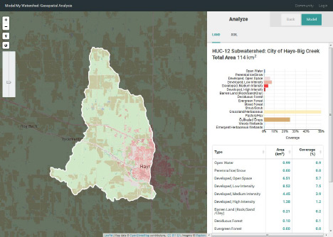
In the analyze pane at the right of the screen, you can view the land use and soil type in both tabular and graphical form. (The table is below the graph. If you cannot see it, scroll down.) Use the tabs at the top right of the pane to switch between land use and soil type. You can sort the tabular data by type, area, or coverage percent. The bar graph coloring will match up with the colors assigned by the National Land Cover Database and can be used as a legend for the land cover and soil group overlays. The title at the top of the analyze pane will list the name of the area (if selected by boundary) and the total size of the area. You can still change the map zoom and overlays in the map pane. Try turning on the NLCD overlay to compare the layout of land covers on the map to the percent of each land cover in the area. To see a larger area of the map, the analyze pane can be minimized by clicking the arrow in the upper right of the pane.

If you realize you made a mistake in selecting your area, hit the back button next model button at the top right of the page. You will be taken back to the choose area of interest screen. To clear the map and select something new, click the teal “Reset” button at the top of the screen. If you are happy with the area you selected, you can move on to modeling and modifying the area by clicking the teal “Model” button on the upper right pane.

Once you have entered the modeling mode, the application will show tabs at the top of the screen for the current conditions and a new scenario where you can modify the landscape by changing the land cover type or applying conservation practices.The model tab will now be filled out with predicted amounts of runoff and stream water quality. The runoff quantities are calculated using a combination of the T​R-55 r​unoff model developed by the US Department of Agriculture and the Small Storm Hydrology Model for Urban Areas developed by Robert Pitt for a single 24-hour rain storm. The water quality parameters are calculated using the EPA's S​TEP-L ​water quality model. For more information on the specifics of these calculations, see other documentation. The runoff tab in the model output pane shows the partitioning of the rainwater into runoff, infiltration, and evapotranspiration as a stacked bar graph. In the water quality tab, you will see both tabular and graphical data showing predicted water quality for any streams in the selected area. Because the model is running with real data on your custom area, it make take some time for the model to run and you may see a loading icon. (It is generally very fast with good internet connection.) The entire model output pane can be minimized by clicking on the arrow in the upper right of the pane.

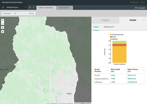
When you begin modeling, you will always begin in the “current conditions” tab. In this tab, you see the analysis and resulting model of the land exactly as it is. The only thing that can be changed in the current conditions tab is the quantity of rainfall to model.

To begin making changes to the landscape, click on the “new scenario” tab at the top of the screen. To start this looks exactly like the “current conditions” tab but with two tool boxes in the upper left, one for land cover and another for conservation practices. Each of these is a free-hand drawing tool to modify the current land use. The model output pane also changes to show the original results from the “current conditions” tab and the modified results as you change the landscape. (The analysis pane will not change.) Select a land use or conservation practice from the toolboxes at the top of the screen and then click points on the map to draw an area over which to apply it. As soon as you add a new land use or conservation practice, the model will re-run in the background to calculate what has changed and all of the plots will be updated. You will see loading icons again in the model pane as this happens. Remember that you can minimize the model output pane to give more screen space to work on landscape modifications. See other documentation for an explanation of how the runoff and water quality contributions of conservation practices are calculated.

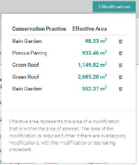
As you add modifications, you can see details about amount of area modified by clicking on any modification box. You can also see a list of all of the modifications you made in the scenario by clicking on the space in the upper right of the map pane where it says “x modifications.” This gives a sort of “shopping cart” of modifications grouped by the type of modification. You can delete any modification by clicking the trashcan next to it. If it helps to decide where to make changes, you can still use the small globe icon to select which overlays to display on the map.

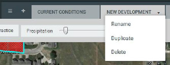
You can create many possible scenarios of landscape modification by clicking on the “+” next to the current conditions tab. This opens up a new tab with no modifications on it. You can also make a copy of one scenario and further modify it by clicking on the arrow on the scenario tab and selecting “duplicate.” Scenarios can be renamed, deleted, and, if you are logged in, shared through the same menu. To help sort through many scenarios, click on the three-lined “hamburger” button next to the “Untitled Project” tab.

Once you have created several scenarios, you can compare all of them by clicking “Compare” in the upper right or the tab bar. This gives a side-by side comparison of all of the scenarios along with the original conditions before any modifications. It also shows what the partitioning would be if the landscape were 100% forested. This 100% forested condition will give the maximum amount of infiltration for the landscape, given its soils. At the top is a map showing the original area and modifications. Below that you can select which type of model output you would like to compare. The same model will apply to all scenarios. At the bottom of the screen there is a list of all the modifications made in each scenario. To scroll through many scenarios, use the arrows on the bottom right of the screen. To return to your scenarios, click the arrow next to “Navigate Scenarios” in the bottom left of the screen.

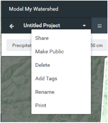
At any time while working, you can name and save your work by clicking on the top left “Untitled Project” tab. You can also make the project publicly accessible to anyone with a link to it, add tags so it can easily be found, print out the maps and graphs, or embed the work into the ITSI portal. Note that this only works if you logged in when you entered the application (and embedding in the ITSI portal requires logging in through the ITSI portal). If you have made your project publicly accessible and given someone the link, they will be able to view all of your scenarios and results. They will not, however, be able to modify it. Any public project can be made private again from the same menu.